Chapter 2
This chapter is about multiarmed bandits (MAB).
There are two kinds of feedbacks to a RL agent:
Evaluative feedback: how well did it act (a score).
Instructive feedback: best action it could do (a correct answer)
In MAP, the environment is a Markov chain, and thus the past does not influence the future. This makes it easy.
This is called nonassociative learning.
In general,
\[Q_t(a) \approx q_*(a) = \mathbb{E}(R_t | A_t = a)\]
$Q_t(a)$ is the estimate of $q_*(a)$, estimated at time $t$. It is updated as time goes on, hopefully approaching $q_*(a)$ better and better.
The greedy strategy is
\[A_t = \underset{a}{\operatorname{argmax}}Q_t(a)\]
The key is to estimate $Q_t$ accurately. There are several ways.
Sample average
\[Q_t(a) = \frac{\text{total reward from choosing a}}{\text{times of choosing a}} = \text{average reward from choosing a so far}\]
which gives the update rule
\[Q_{n+1} = Q_n + \frac{1}{n}(R_n - Q_n)\]
it is cast in the general form:
\[\text{new estimate} = \text{old estimate} + \text{step size} \times \text{error}\]
The number $\alpha = \frac 1 n$ is the step size for the sample average method, and it quantifies how much the latest error would affect the new estimate.
Early experience matters a lot, later a little. Like old people that are hard to change.
Exponential recency weighted average
Set $\alpha$ constant, then we get
\[Q_{n+1} = Q_n + \alpha(R_n - Q_n)\]
By stochastic approximation theory, there's a theorem:
Theorem: If \(\sum_{n}^{} \alpha_n = \infty , \sum_n \alpha_n^2 < \infty \), then almost surely \(Q_n \to \text{true value}\)
For sample average, $\alpha_n = 1/n$ gives convergence. It's just the strong law of large numbers.
For constant $\alpha$, it does not converge, but that's the point, since it's supposed to respond to change.
Practically, this theorem is useless since the convergence is too slow.
Optimistic Initial Bias
By setting $Q_1$ big, the agent is encouraged to explore at first. It would keep trying the untried options, get disappointed, try another, get disappointed, until all have been tried. It's a cheap trick that works well enough, when you want the agent to explore more at the beginning.
Does not work for nonstationary bandits.
Upper Confidence Bound (UCB)
\[A_t = \underset{a}{\operatorname{argmax}}\left[ Q_t(a) + c\sqrt{\frac{\log t}{N_t(a)}} \right] \]
The parameter $c \ge 0$ measures the exploration rate of the agent. $c=0$ is completely greedy, and lage $c$ is explorative.
The term $\log t$ means that any option that's unexplored for long would appear more and more attractive, but older agents would be slower to have their curiosity awakened than newborns.
It's very good for MAB, but not so much for other problems.
Boltzmann Distribution
Turn the problem into a problem of thermodynamics!
Let the options be states and let $-H_t(a)$ be the energy lever of state $a$ at time $t$, then the Boltzmann distribution is
\[\pi_t(a) = \frac{e^{H_t(a)}}{\sum_a e^{H_t(a)}}\]
(side note: $H$ means Hamiltonian)
Then we can choose like particles choose in statistical mechanics:
\[Pr(A_t = a) = \pi_t(a)\]
A big $H_t(a)$ means a low energy, thus energetically favored, and chosen more often.
The energy levels are updated by:
\[\begin{cases}H_{t+1}(A_t) = H_t(A_t) + \alpha(R_t - \overline{R_t}) (1-\pi_t(A_t)),\\H_{t+1}(a) = H_t(a) + \alpha(R_t - \overline{R_t}) (-\pi_t(a))\end{cases}\]
Notice that since \(\sum_a \pi_t(a) = 1\), we have \(\sum_a H_{t+1}(a) = \sum_a H_t(a)\), so this keeps the normalization of the energy levels (as in physics, the absolute energy doesn't matter, only the relative energy matters).
Conclusion
There are several ways to do the MAB problem, and they generalize to full RL problems. UCB works great for MAB but not so great for general RL.
Gittins Index, Bayesian, posterior sampling, are some methods that can give exact optimal strategies. They are too hard to calculate but might be approximable.
Exercises
2.1: Probability of choosing greed is \((1-\epsilon) + \frac{\epsilon}{n}\)
2.2: 4 and 5 are definitely explore. All others are unsure.
2.3: In the limit, the optimal action is chosen \((1-\epsilon) + \frac{\epsilon}{n}\) of the times.
For \(n=10\) case, we have \(\epsilon = 0.1, p = 0.91; \epsilon = 0.01, p = 0.991\).
2.4: \(Q_{n+1} = \prod_{i=1}^{n} (1-\alpha_i) Q_1 + \sum_{j=1}^{n} R_j \alpha_j \prod_{i=j+1}^{n}(1-\alpha_i) \)
2.5: The exp recency dominates at around 1000 steps, and achieves consistently 0.8 probability of choosing the right answer.

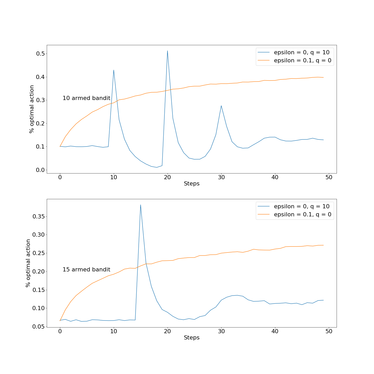
2.6: As seen in the picture, the spike happens because the optimistic agent spends the first 10 steps happily exploring (and disappointed every time), then after all the disappointments, it has explored all of them and has a good idea of which one is the best, and chooses that one. Then it gets disappointed again because even the best one is still not living up to the expectation, so the agent starts exploring again. After 20 steps, each arm has been tried twice, and so the agent would have an even better idea of which one is the best and starts using that option more often, and after being disappointed a third time, doesn't get so disappointed that it would start exploring all over again, and that's why theer's a second "plateau".

This is confirmed when we set the arm number to 15, and witness that the spike and the plateau gets moved back to 15 and 30.
It's also expected that a more optimistic agent would experience more such cycles of highs of explorations and lows of disappointment, so we added the optimism up to 10 and indeed witnessed more spikes.

2.7: \(o_0 = 0, o_{n+1} = o_n + \alpha(1- o_n)\), thus \(o_n = 1-(1-\alpha)^n\), \(\beta_n = \alpha/o_n\)
\[Q_{n+1} = Q_n + \frac{\alpha}{1- (1-\alpha)^n} (R_n - Q_n)\]
so \(Q_2 = R_1\) removes initial bias, and at large \(n\), \(\beta_n \to \alpha\), so it approaches exponential recency-weighted average.
2.8: We see that the higher \(c\), the more exploration the agent does, and the sharper the spike is. The reason is the same as in 2.6: more exploration = more spikiness.

2.9: If the options are \(\{0, 1\} \) then
\[Pr(A_t = 1) = \frac{1}{1+e^{-(H_t(1 ) - H_t(0))}} = S(H_t(1) - H_t(0))\]
where \(S(x) = \frac{1}{1 + e^{-x}}\) is the sigmoid function.
2.10: Nonassociative case: doesn't matter. Expected value is 0.5. Associative case: obvious, expected value is 0.55.
2.11: This exercise was quite a beast. I ran the test with each bandit algorithm repeated 2000 times, and averaged over them. For each run, the algorithm faces a bandit problem and plays it 2e5 times, and only the last 1e5 times are considered to fully remove the effect of initial explorations and concentrate only on long-term behavior.
The results are plotted. They took about 6 hours to compute.

TODO: study the box at page 38-40.


No comments:
Post a Comment