- Sutton & Barto, rest of Chapter 4
- Sutton & Barto, Chapter 5
In this post we do chapter 4.
\[v_\pi(s) = \sum_a \pi(a|s) \sum_{s', r}p(s', r|s, a)(r + \gamma v_\pi(s'))\]
And that looks like a fixed-point problem, and can be solved by iterative updating: start with some $v_0 : S^+ \to \mathbb{R}$, with the condition that it is $0$ on the terminal state (if it exists). Then, for any $s\in S$, update it by
\[v_{n+1}(s) = \sum_a \pi(a|s) \sum_{s', r}p(s', r|s, a)(r + \gamma v_n(s'))\]
Theorem: If $v_\pi$ exists, then $v_n \to v_\pi$.
Instead of updating $v_n$ all at once, it can be updated state-by-state, sweeping through the state space $S$, that is, "updating the array in place". By another theorem, updating in place also converges to $v_\pi$. And it usually converges faster.
Ex. 4.1: -14, 0
Ex. 4.2: Since state 15 is inaccessible from the original states, so the values of the original states are unchanged (intuitively, state 15 is "invisible" for any player not in it, so it might as well not exist).
In such case, $v_\pi(15) = 1/4 (-22-20-14 + v_\pi(15)) = -56/3$
If state 15 is accessible, it'd make things a lot more complicated. I modified the program and got these:
Ex. 4.3: From modifying the fixed-point equation in ex. 3.13, we have
\[q_{n+1}(s, a) = \sum_{s', r} p(s', r | s, a)\left[ r + \gamma \cdot \sum_{a'} \pi(a' | s') q_n (s', a') \right] \]
A lot of RL algorithms are made from this simple change from a fixed-point formula to a step-by-step formula. Convergence is rarely a problem, but speed of convergence usually is. In fact, many good numerical algorithms are downright divergent...
$$\text{policy } \pi_1 \to \text{value } v_{\pi_1} \to \text{new greedy policy } \pi_2 \text{ based on } v_{\pi_1} \to \cdots$$
loop until the policy stabilizes: $\pi_n = \pi_{n+1}$, at which point we actually get the optimal policy.
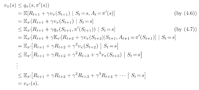
Theorem (Policy Improvement): If $\pi, \pi'$ are deterministic policies, such that, $\forall s\in S, q_{\pi}(s, \pi'(s))\ge v_{\pi}(s)$, then $v_{\pi} \succeq v_{\pi'}$. If all the $\ge$ are $=$, then $v_{\pi} = v_{\pi'}$, and if one of the $\ge$ is $>$, then $v_{\pi} \succ v_{\pi'}$
Proof: see p78 of the book:
Corollary: If $\pi'$ is the greedy strategy guided by $v_\pi$, then $\pi' \succeq \pi$. If $\pi' = \pi$, then $\pi$ is optimal, since it satisfies the Bellman equation.
Thus we obtain the policy estimation algorithm:
Since there are only finitely many deterministic policies, this terminate in finite time.
Ex. 4.4: There are several ways to modify the code:

I took this result from How to Gamble If You Must (2008), by Kyle Siegrist.
Ex. 4.8: I don't know...
Ex. 4.9: As we explained earlier, $p=0.55$ gives the timid strategy, and $p = 0.25$ gives the bold strategy. Note that it's not literally the bold strategy, but that's just because the optimal strategy is not unique.
Back in Value Iteration, we truncated the $\text{find } v_\pi$ step to one sweep. This can be truncated even further. We can only sweep at only one state, instead of all the states. As long as all the states are sweeped infinitely often, $\pi$ would still converge to the optimum.
This is practically necessary when the state space is too big or not known. It has other benefits too: We can select the most promising states to update first, or update the states in an efficient order, or skip over states that we are sure won't be relevant in the optimal behavior.
And if it's an online learning problem, we can updates the states as the agent visits them. These states are usually the most relevant. This kind of focusing is a repeated theme in reinforcement learning.
There's an adversarial sense to GPI: on one hoof, Policy Evaluation calculates $v_\pi$ and use that to demonstrate that $\pi$ is not optimal; on the other hoof, Policy Update uses $v_\pi$ to create a better policy that will be closer to optimal. When both sides cannot improve, they shake hooves and achieve optimality.
Linear programming methods can also be used to solve MDPs. but for the largest problems, only DP methods are feasible.
On problems with large state spaces, asynchronous DP methods are often best.
Dynamic Programming (DP)
Define: DP: a collection of algorithms to compute optimal policies for an MDP model of the environment.
Classical DP algorithms are of limited utility in reinforcement learning both because of their assumption of a perfect model and because of their great computational expense, but they are still important theoretically. DP provides an essential foundation for the understanding of the methods presented in the rest of this book. In fact, all of these methods can be viewed as attempts to achieve much the same effect as DP, only with less computation and without assuming a perfect model of the environment.Basically, can't solve Bellman, can't do classical DP, put them up as unachievable ideals and opt for more practical algorithms that can approximate them.
Prediction Problem/Policy Evaluation
Given a policy $\pi$, calculate its value functions $p_\pi, v_\pi$. Theoretically,\[v_\pi(s) = \sum_a \pi(a|s) \sum_{s', r}p(s', r|s, a)(r + \gamma v_\pi(s'))\]
And that looks like a fixed-point problem, and can be solved by iterative updating: start with some $v_0 : S^+ \to \mathbb{R}$, with the condition that it is $0$ on the terminal state (if it exists). Then, for any $s\in S$, update it by
\[v_{n+1}(s) = \sum_a \pi(a|s) \sum_{s', r}p(s', r|s, a)(r + \gamma v_n(s'))\]
Theorem: If $v_\pi$ exists, then $v_n \to v_\pi$.
Instead of updating $v_n$ all at once, it can be updated state-by-state, sweeping through the state space $S$, that is, "updating the array in place". By another theorem, updating in place also converges to $v_\pi$. And it usually converges faster.
Ex. 4.1: -14, 0
Ex. 4.2: Since state 15 is inaccessible from the original states, so the values of the original states are unchanged (intuitively, state 15 is "invisible" for any player not in it, so it might as well not exist).
In such case, $v_\pi(15) = 1/4 (-22-20-14 + v_\pi(15)) = -56/3$
If state 15 is accessible, it'd make things a lot more complicated. I modified the program and got these:
0 -14.685 -20.883 -22.893
-15.007 -19.173 -21.071 -20.902
-21.847 -21.928 -19.327 -14.743
-24.607 -23.367 -15.564 0
Which shows that the addition of the "sink" really dragged down the values all around the board, especially near that spot. If we take the difference of values before and after adding that sink, we get:-27.367
0 -0.685 -0.883 -0.893
-1.007 -1.173 -1.071 -0.902
-1.847 -1.928 -1.327 -0.743
-2.607 -3.367 -1.564 0
Ex. 4.3: From modifying the fixed-point equation in ex. 3.13, we have
\[q_{n+1}(s, a) = \sum_{s', r} p(s', r | s, a)\left[ r + \gamma \cdot \sum_{a'} \pi(a' | s') q_n (s', a') \right] \]
A lot of RL algorithms are made from this simple change from a fixed-point formula to a step-by-step formula. Convergence is rarely a problem, but speed of convergence usually is. In fact, many good numerical algorithms are downright divergent...
This series is divergent, therefore we may be able to do something with it.
---- Oliver Heaviside
Policy Improvement
The idea is simple:$$\text{policy } \pi_1 \to \text{value } v_{\pi_1} \to \text{new greedy policy } \pi_2 \text{ based on } v_{\pi_1} \to \cdots$$
loop until the policy stabilizes: $\pi_n = \pi_{n+1}$, at which point we actually get the optimal policy.
Theorem (Policy Improvement): If $\pi, \pi'$ are deterministic policies, such that, $\forall s\in S, q_{\pi}(s, \pi'(s))\ge v_{\pi}(s)$, then $v_{\pi} \succeq v_{\pi'}$. If all the $\ge$ are $=$, then $v_{\pi} = v_{\pi'}$, and if one of the $\ge$ is $>$, then $v_{\pi} \succ v_{\pi'}$
Proof: see p78 of the book:

Corollary: If $\pi'$ is the greedy strategy guided by $v_\pi$, then $\pi' \succeq \pi$. If $\pi' = \pi$, then $\pi$ is optimal, since it satisfies the Bellman equation.
Thus we obtain the policy estimation algorithm:
Since there are only finitely many deterministic policies, this terminate in finite time.
Ex. 4.4: There are several ways to modify the code:
- Order the actions $A$, so that whenever there's a tie in the argmax during Policy Improvement, always take the lowest-ordered action.
- Store all policies and terminate when the policy obtained has been obtained before.
- Store all the policy valuations and terminate when the valuation improvement is too small.
Ex. 4.5: In Policy Evaluation, use the line
$$Q(s, a) \leftarrow \sum_{s', r} p(s', r|s, a)[r + \gamma Q(s', \pi(s'))]$$
and in Policy Improvement, use
$$\pi(s) \leftarrow \underset{a}{\operatorname{argmax}} Q(s, a)$$
Ex. 4.6:
- No change.
- Change one line: \[V(s) \leftarrow \frac{\epsilon}{|A(s)|} \sum_{a\in A(s)}\sum_{s', r} p(s', r | s, a) \left[ r + \gamma V(s') \right] + (1-\epsilon)\sum_{s', r} p(s', r | s, \pi(s)) \left[ r + \gamma V(s') \right] \]
- For returning $\pi_*$, change to "$\pi$ but $\epsilon$-softened". That is, for all $s\in S, a \in A(s)$, if $a \neq \pi(s), then \pi_*(a | s) = \epsilon / |A(s)|$, else, $\pi_*(a | s) = (1-\epsilon) + \epsilon / |A(s)|$.
Ex 4.7: It's quite easy to modify the provided code in the github repository to get:

Note that in the optimal policy (closely approximated by policy 4), there are "islands of blue" that are meant to avoid extra parking fees.
Value Iteration
In the policy evaluation, instead of sweeping through the state space until $V$ becomes stabilized, ie does not change by more than a small number $\theta$, before updating $\pi$, we can instead be impatient and update $\pi$ immediately after one sweep. The resulting algorithm is the "value iteration".
More generally, we can do several sweeps, before doing a value iteration.
Theorem: All of these algorithms converge to an optimal policy for discounted finite MDPs.
Ex. 4.10: \[q(s, a) = \sum_{s', r} p(s', r | s, a) [r + \gamma \max_{a'}q(s', a')]\]
Gambler's Problem
According to Inequalities for Stochastic Processes; How to Gamble if You Must, by Lester E. Dubbins and Leonard (Jimmie) Savage, the problem has many different optimal deterministic strategies, and so it's unsurprising that the DP converges to rather odd strategies.
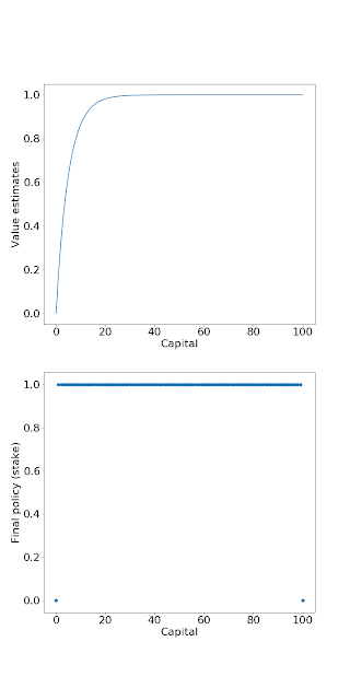
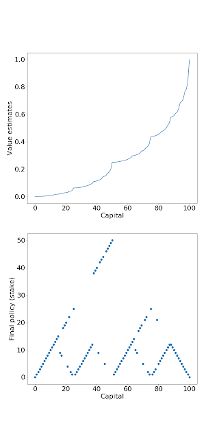
The result from the book is that, if the gambling is unfavorable ($p < 0.5$), then use the bold strategy: gamble $\max(s, 100-s)$, and if favorable, gamble only $\$1$ always. Basically, if the odds are bad, be bold; if the odds are good, be timid. If the odds are even, then it literally doesn't matter.
I took this result from How to Gamble If You Must (2008), by Kyle Siegrist.
Ex. 4.8: I don't know...
Ex. 4.9: As we explained earlier, $p=0.55$ gives the timid strategy, and $p = 0.25$ gives the bold strategy. Note that it's not literally the bold strategy, but that's just because the optimal strategy is not unique.


Asynchronous DP
Remember the loop of D: $$\cdots \to \text{find } v_\pi \to \text{find greedy } \pi \to \cdots$$
This is practically necessary when the state space is too big or not known. It has other benefits too: We can select the most promising states to update first, or update the states in an efficient order, or skip over states that we are sure won't be relevant in the optimal behavior.
And if it's an online learning problem, we can updates the states as the agent visits them. These states are usually the most relevant. This kind of focusing is a repeated theme in reinforcement learning.
Generalized Policy Iteration (GPI)
The loop thing I described is technically called GPI. Almost any reinforcement learning method is some sort of GPI.There's an adversarial sense to GPI: on one hoof, Policy Evaluation calculates $v_\pi$ and use that to demonstrate that $\pi$ is not optimal; on the other hoof, Policy Update uses $v_\pi$ to create a better policy that will be closer to optimal. When both sides cannot improve, they shake hooves and achieve optimality.
Efficiency of DP
DP may not be practical for very large problems, but compared with other methods for solving MDPs, DP methods are actually quite efficient...Time complexity of DP for calculating optimal policy is polynomial in the number of states and actions.
Linear programming methods can also be used to solve MDPs. but for the largest problems, only DP methods are feasible.
On problems with large state spaces, asynchronous DP methods are often best.


No comments:
Post a Comment