MC methods in this chapter differ from the DP methods in two major ways. First, they operate on sample experience, and thus can be used for direct learning without a model. Second, they do not bootstrap. That is, they do not update their value estimates on the basis of other value estimates.
These two differences are not tightly linked, and can be separated. In the next chapter we consider methods that learn from experience, like Monte Carlo methods, but also bootstrap, like DP methods.
Monte Carlo Estimation of $v_\pi$ and $p_\pi$
This can be thought of as a generalization of the DP method. There's still the $v_\pi \to \pi \to v_\pi$ loop, but now, the Policy Evaluation step is no longer a matter of explicit calculation, but a stochastic guess my Monte Carlo method.
For estimating $v_\pi(s)$, just start at state $s$, then do lots of rollouts from $s$, until satisfied. For estimating $p_\pi(s, a)$, similarly do rollouts from $s$ with action $a$. If we have a model of the world, so we can rollout from $s$, then $v_\pi$ is amenable to MC, else, $p_\pi$ ca be better, especially in case of online learning.
The problem with using deterministic policies is that there'd be no exploration of many state-action pairs. To maintain exploration, one method is using exploring starts: Star the episodes with a state–action pair, and let every pair have a nonzero probability of being selected as the start. Another method is to consider only stochastic policies, where any allowable state-action pair has nonzero probability.
First-visit and every-visit
The first-visit MC evaluation is simple enough. Here, $V$ is the iterative approximation of $v_\pi$, and $Returns$ is a list of lists: $\forall s\in S, Returns(s) = \text{a list of returns from episodes starting at }s$

The every-visit MC is similar. Just remove the line about "Unless $S_t$ appears in $S_0, ..., S_{t-1}$".
The first-visit MC converges as $n^{-1/2}$, where $n$ is the number of times of visiting the state $s$, by the law of large numbers. It's the same for every-visit MC, but the proof is harder.
Blackjack!
In a game of Blackjack, because there's hidden information (on the dealer's side, and in the deck), calculating the transition function $p(s', r | s, a)$ would be quite difficult, making Policy Evaluation difficult too. But if we use Monte Carlo, then we don't need to evaluate $p$ explicitly.
 |
| Let's play! |
Ex. 5.1: Because it's a very good situation when the player has 20 or 21 points. It's an almost sure win. Because if the dealer has an A, the dealer has more flexibility and thus more likely to win. Because if the player has A, the player is more likely to win.
Ex 5.2: The result would be precisely the same, since in a blackjack episode, there's no way for a state to appear twice. Such games are "accumulative" because the cards are never lost. In general, any card game without card recycling is accumulative.
Bubbles!
The idea is simple: The bubble film is a minimal surface, which means everywhere, its two principal curvatures add up to 0, and by some approximation, if the bubble is not too deformed, it's described by a harmonic function, which satisfies the mean-value theorem:
On any point of the surface, its height equals the average of all the points on a circle around that point.
Question: if we fix the boundary of the surface (like after dipping a bubble blower into soup), what's the shape of the bubble?
Idea! If we consider this a game, and the game states are the points on the surface, the end states are the points on the blower, and the game strategy is "take a step of size $\epsilon$ in a random direction", then the valuation of the strategy converges to the shape of the bubble, when $\epsilon$ is small enough.
(On-policy) Monte Carlo Control (Policy Iteration)
We still have the cycle of generalized policy iteration (GPI):
$$\text{policy} \pi \leftrightarrow \text{action value } p_\pi$$
$\pi$ is still greedy like before: $\pi(s) = \underset{a}{\operatorname{argmax}}q(s, a)$.
Except now, we must obtain $p_\pi$ by stochastic simulation, instead of direct calculation. And as mentioned, MC cannot explore well with deterministic policies, so it must be fixed by using exploring starts.
Two assumptions are unrealistic:
- Exhaustive exploring starts. In practice, it's not possible to try out all state-action pairs.
- Perfect evaluation of $p_\pi$. It requires infinitely many MC rollout trials.
To deal with perfect evaluation, we simply approximate by:
- Do many trials until the expected error is small enough.
- Don't bother evaluating accurately, and just use value iteration, like back in DP.
Don't evaluate accurately
For MC, it is natural to alternate between evaluation and improvement episode-by-episode:
After each episode, the observed returns are used for policy evaluation, and then the policy is improved greedily at all the states visited in the episode.The algorithm is then called Monte Carlo with Exploring Starts (MCES).

Ex. 5.4: Replace $Returns$ with $EpisodeCount$, and replace some lines with these lines at the appropriate places: $$EpisodeCount(s, a) \leftarrow 0 \text{ for all } s\in S, a \in A(s)$$$$EpisodeCount(S_t, A_t) \leftarrow EpisodeCount(S_t, A_t) + 1 $$$$n \leftarrow EpisodeCount(S_t, A_t)$$ $$Q(S_t, A_t) \leftarrow Q(S_t, A_t) + \frac 1 n (G - Q(S_t, A_t))$$
Open conjecture: The MCES converges to optimal policy.
TODO: Prove this conjecture.
The book uses MCES to calculate a strategy for a simplified version of Blackjack. It looks similar to Thorp's basic strategy from Beat the Dealer (1966).

Don't do exploring starts
The trouble with deterministic policies is that they are bad for exploring. You can't explore if you know exactly what you should do! Exploring starts are supposed to fix this, by forcing you to take the first step randomly.
The point of exploring starts is to make sure that we try out every state-action pair infinitely many times. If we don't have time to explore all the things all at once right at the start, we can just use some other trial-scheduling to ensure that every state-action pair is tried infinitely often.
Two general ways to do this are called on-policy and off-policy.
On-policy methods mean that the program iteratively improve a policy $\pi$ until it's approximately optimal, then it's returned.
Off-policy methods mean that the program iteratively improve a behavior policy $\pi$ to generate data about the world, then at the last step, use that policy as a guide to generate a target policy $\pi'$.
On-policy methods are simpler. Off-policy methods are harder and are slower to converge. On the other hoof, off-policy methods are more powerful and general.
On-policy
Define: a policy $\pi$ is soft iff $\forall s\in S, a\in A(s), \pi(a | s) > 0$. It's $\epsilon$-soft iff $\forall s\in S, a\in A(s), \pi(a | s) \ge \epsilon/|A(s)|$.
Note that, given a value function, the corresponding $\epsilon$-greedy policy is the greediest policy among all corresponding $\epsilon$-soft policies.
On-policy methods generally use soft policies, so that exploration is always on. The softness tends to decrease as time goes on, though. Just like simulated annealing.
Theorem: Any $\epsilon$-greedy policy $\pi'$ with respect to $q_\pi$ improves over any $\epsilon$-soft policy $\pi$.
A softer Equestria
Instead of using $\epsilon$-soft policies, we can use an $\epsilon$-softened world. Basically, make a world where after every move, with $1-\epsilon$ probability it behaves like the old world, and $\epsilon$ probability it picks a random action and then behaves like the old world.
Off-policy
The prediction problem
An exploration team was sent to the game and played many episodes using policy $b$. They came back with their game records. You want to know, based on those game records, how well a policy $\pi$ would do. This is the prediction problem.
Coverage assumption: $\forall s\in S, a\in A(s)$, if $\pi(a | s) > 0$ then $b(a | s ) > 0$.
That is, the team must have tried more than you dare to.
Importance Sampling
The importance sampling method. What we want to estimate is an expectation \[v_\pi(s) = \mathbb{E} [G_t | S_t = s, \pi] = \sum_{\text{continuations } S_t = s, A_t, \cdots, S_T} G_t \cdot Pr(A_t, \cdots, S_T | S_t = s, \pi)\]
But we only have $G_t$ sampled using policy $b$. To fix this, we define a new random variable over the policy $b$: \[\rho_{t:T-1} = \prod_{k=t}^{T-1} \frac{\pi(A_k | S_k)}{b(A_k | S_k)} \] That gives \[Pr(A_t, \cdots, S_T | S_t = s, \pi) = \rho_{t:T-1} Pr(A_t, \cdots, S_T | S_t = s, b)\] Thus, \[v_\pi(s) = \mathbb{E}[\rho_{t:T-1}G_t | S_t = s, b]\]
Now we consider estimating $v_\pi$ by the running MC with $b$ for many episodes. For notational convenience, we concatenate all episodes together into one long sequence indexed by time $t$, and define $T(t)$ to be the end of the episode that $t$ is in.
Define \(J(s) = \{t : S_t = s\} \) if we are doing every-visit MC, and \(J(s) = \{t : S_t = s \text{ for the first time in the episode of }t \} \) if first-visit MC.
In practice, every-visit methods are often preferred because they remove the need to keep track of which states have been visited and because they are much easier to extend to approximations.
There are two ways to estimate over all such samples: weighted and unweighted/ordinary.
Ordinary Importance Sampling:\[V_{ord}(s) = \frac{\sum_{t\in J(s)} \rho_{t: T(t)-1} G_t}{|J(s)|} = \frac{\sum_{t\in J(s)} \rho_{t: T(t)-1} G_t}{ \sum_{t\in J(s)} 1} \] Weighted Importance Sampling: \[V_{weighted}(s) = \frac{\sum_{t\in J(s)} \rho_{t: T(t)-1} G_t}{\sum_{t\in J(s)} \rho_{t: T(t)-1}} = \frac{V_{ord}(s)}{\frac{1}{|J(s)|} \sum_{t\in J(s)} \rho_{t: T(t)-1}}\]
It's clear that $V_{ord}(s)$ is an unbiased estimator of $v_\pi(s)$, and $V_{weighted}(s)$ is biased, but as $|J(s)|\to\infty$, we have \[V_{weighted}(s) \to \frac{1}{\mathbb{E}_b[\rho_{t:T-1} | S_t=s]} v_\pi(s)\] and to show that it's also unbiased at this limit, we prove that the denominator is one.
\begin{equation} \begin{split} \mathbb{E}_b[\rho_{t:T-1} | S_t=s] ={} & \sum_{S_t = s, A_t, \cdots , A_{T-1}, S_T = terminal} \rho_{t:T-1}\prod_{k =t}^{T-1} b(A_k | S_k)p(S_{k+1} | S_k, A_k) \\ ={} & \sum_{S_t = s, A_t, \cdots , A_{T-1}, S_T = terminal}1 \prod_{k=t}^{T-1} \pi(A_k | S_k)p(S_{k+1} | S_k, A_k) \\ ={} & \mathbb{E}_\pi [1 | S_t = s] \\ ={} & 1 \end{split} \end{equation}
In practice, the weighted estimator usually has dramatically lower variance and is strongly preferred.Ex. 5.5: First visit: 10. Every-visit: 5.5
Ex.5.6: \[Q(s, a) = \frac{\sum_{t\in J(s)} \rho_{t+1: T(t) - 1}G_t}{ \sum_{t\in J(s)} \rho_{t+1: T(t) - 1}}\]
Ex.5.7: TODO: solve this.
Ex.5.8: The variance is still infinite. Consider what happens after finishing episode $i$. Let $C$ be the number of visits to $s$ before episode $i$, and let $C'$ be the sum of $\rho_{t: T-1} G_t$ before episode $i$, then we calculate the variance of the estimator after episode $i$: $$V_i(s) = \frac{C' + \sum_{k=1}^{n-1} \rho_{k: n-1}G_k}{C + n}$$
The variance is infinite, since we have $$\mathbb{E}_b (V_i(s)^2) = \cdots = \sum_{n=1}^\infty \left( \frac{2^{n+1} - 2 + C'}{C+n}\right)^2 \frac{9^{n-1}}{20^n}\sim \frac 4 9 \sum_{n=1}^\infty \frac{1}{n^2}\left( \frac 9 5 \right)^n = \infty$$
Ex 5.9: Add these lines at appropriate places: $$N(s) \leftarrow 0, \text{ for all } s\in S$$ $$N(S_t)\leftarrow N(S_t) + 1$$ $$V(S_t) \leftarrow V(S_t) + \frac{1}{N(S_t)} (G - V(S_t))$$
Ex. 5.10: Trivial.
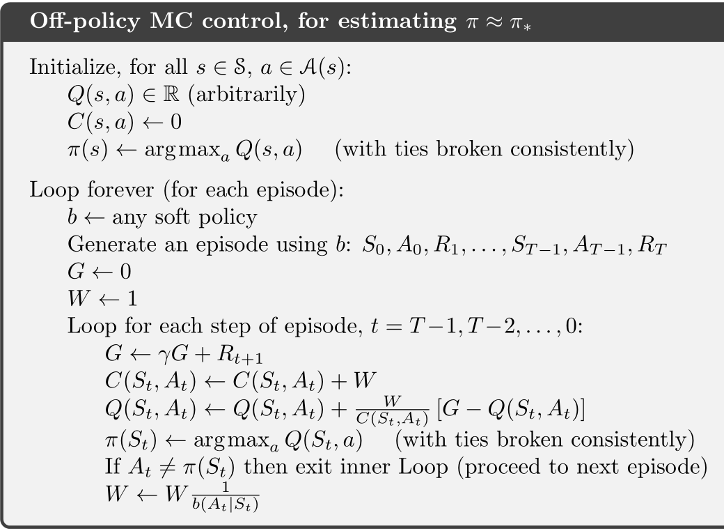
Off-policy MC Control
I can't explain much more about this algorithm, other than noting that yes, indeed, it works, but doesn't seem to be a very efficient one.The reason that only the greedy tail is preserved is that $\pi$ is always greedy, so any action that's not greedy, $\pi(a | s) = 0$ and that makes $W= 0$ for the rest of the episode, which makes it pointless to keep evaluating beyond the greedy tail.
Ex. 5.11: Because if $\pi = 0$ if not greedy, and $\pi = 1$ if greedy.
Ex. 5.12: not TODO.
Extra credit stuff
Practical convergence is all about reducing variance. Weighted importance-sampling has less variance, so that's good. There are more tricks.
Another way to reduce variance is by Section 5.9 method of per-decision importance sampling.
Ex. 5.13: Mimic equation (5.13).
Ex. 5.14: For converting equation (5.10) into $Q(s, a)$, simply replace every $\rho_{t: i}$ with $\rho_{t+1: i}$, with the caveat that $\rho_{t+1: t} = 1$.
For modifying the algorithm... well, I really don't want to deal with that!!


No comments:
Post a Comment