Let's read: Sutton's RL, week 5 to 6, chap 6

In this post we read chapter 6, about Temmporal Difference (TD) learning:

If one had to identify one idea as central and novel to reinforcement learning, it would undoubtedly be TD learning... The relationship between TD, DP, and MC methods is a recurring theme in RL.

TD learning is a combination of MC and DP.

• Like MC, TD methods can learn directly from raw experience without a model of the environment’s dynamics.
• Like DP, TD methods update estimates based in part on other learned estimates, without waiting for a final outcome (they bootstrap).
• Bootstrapping: using a guess to make a better guess.
• The master of RL must master TD, MC, DP as one and use them in many combinations.

We consider the origin of the three algorithms of MC, DP, and TD, as used in the policy evaluation problem: given $\pi$, find $v_\pi$.
\begin{equation}\begin{split}v_\pi(s) ={} & \mathbb{E}_\pi[G_t | S_t = s] \quad \text{MC, statistical, non-bootstrap}\\ ={} & \mathbb{E}_\pi[R_{t+1} + \gamma v_\pi (S_{t+1}) | S_t = s]\quad \text{TD(0), statistical, bootstrap}\\ ={} & \sum_{a, r, s'} [r + \gamma v_\pi(s')]\pi(a | s) p(s', r | s, a) \quad \text{DP, calculational, bootstrap}\end{split} \end{equation}
$\mathbb{E}$ signals statistical methods: try a bunch of episodes, then extract values from the episode records by averaging and weighting.

$v_\pi$ signals bootstrapping: to find $v_\pi$, we guess a preliminary $v_\pi$, then use that to improve upon the guess, cycle until the guess is good enough.

$p(s', r | s, a)$ signals modelling the environment: if the agent wants to do DP, it must know what the environment is like. Without it, the agent must resort to model-free learning, such as in MC and DP.

TD

TD(0)

TD(0) is obtained by statistically approximating $$V(S_t) = \mathbb{E}_\pi[R_{t+1} + \gamma V(S_{t+1}) | S_t = s]$$ by running many episodes, and updating along the way: \[V(S_t)\leftarrow V(S_t) + \alpha\left[ R_{t+1} + \gamma V(S_{t+1}) - V(S_t) \right] \]

n-step TD

It can be obviously generalized to n-step TD algorithm by expanding out the thing to 

$$V(S_t) = \mathbb{E}_\pi[R_{t+1} + \cdots + \gamma^n R_{t+n+1} + \gamma^{n+1} V(S_{t+n+1}) | S_t = s]$$ so that \[V(S_t)\leftarrow  V(S_t) + \alpha\left[ \sum_{k=0}^{n} \gamma^k R_{t+1+k} + \gamma^{n+1}V(S_{t+n+1}) -V(S_t) \right] \]

Note that due to some silly notational convention, n-step TD method is NOT written as TD(n), and also the 1-step TD method is written as TD(0)... Confusion.

TD-error

Define: TD-error $\delta_t = R_{t+1} + \gamma V(S_{t+1}) - V(S_t) $

As special cases, we have $\delta_{T-1} = R_T - V(S_{T-1}), \delta_T = 0$

The MC-error is related to the TD-error by $$G_t - V(S_t) = \delta_t + \gamma(G_{t+1} - V(S_{t+1}))= \sum_{k=t}^{T-1} \gamma^{k-t}\delta_k$$
This is only approximate if $V$ is updated during the episode. To take the updating into account, we explicitly label the $V$ with time as well, so that \[V_{t+1}(S_t)=V_t(S_t) + \alpha \delta_t \] \[\delta_t = \left[ R_{t+1} + \gamma V_t(S_{t+1}) - V_t(S_t) \right] \]
Then, we have the MC-error related to the TD-error by \begin{equation}G_t - V_t(S_t) = \delta_t + \gamma(G_{t+1} - V(S_{t+1}))= \sum_{k=t}^{T-1} (1 + \gamma\alpha 1_{S_{k+1} = S_k}) \gamma^{k-t}\delta_k\end{equation}
This solves Ex. 6.1.

Ex. 6.2: I guess it's because the TD learning methods are more efficient when encountering familiar situations. In the hint:

Suppose you have lots of experience driving home from work. Then you move to a new building and a new parking lot (but you still enter the highway at the same place). Now you are starting to learn predictions for the new building.

Using TD learning, you can update immediately after noting that you are entering the highway, and then you are done. Using MC learning, you can only update after you get home.

Ex. 6.3: In the first episode, it ended up terminating on the left. The change is $V(A) = 0.45$.
Ex. 6.4: The tradeoff is that high $\alpha$ makes early learning fast, but long-term error big. The best way would be annealing: start high and as time goes on, turn it small.
Ex. 6.5: There's a sweetspot where $V$ is just right, but then the algorithm cannot stay there and starts oscillating around the right point. If the $V$ is initiated somewhat randomly around the right value, then the average RMS error would just be a horizontal line.
Ex. 6.6: It can be calculated by DP, and standard probability. I guess the author used standard probability, since that's how I did it, and the problem is so simple it could be seen at a glance.

SARSA, n-step SARSA, expected SARSA, Q-learning

Instead of evaluating $V$, we evaluate $Q$. It's obvious how to change $V$ to $Q$ in this equation: \[V(S_t)\leftarrow V(S_t) + \alpha\left[ R_{t+1} + \gamma V(S_{t+1}) - V(S_t) \right] \] becomes \[Q(S_t, A_t)\leftarrow Q(S_t, A_t)+ \alpha\left[ R_{t+1} + \gamma Q(S_{t+1}, A_{t+1})-Q(S_t, A_t) \right] \]

This is called SARSA, from $S_t, A_t, R_{t+1}, S_{t+1}, A_{t+1}$.

Similarly, we have n-step SARSA by \[Q(S_t, A_t)\leftarrow  Q(S_t, A_t) + \alpha\left[ \sum_{k=0}^{n-1} \gamma^k R_{t+1+k} + \gamma^{n}Q(S_{t+n}, A_{t+n    }) -Q(S_t, A_t) \right] \]

A small modification of SARSA gives the expected SARSA: \[Q(S_t, A_t)\leftarrow Q(S_t, A_t)+ \alpha\left[ R_{t+1} + \gamma \sum_a \pi(a| S_{t+1}) Q(S_{t+1}, a)-Q(S_t, A_t) \right] \]

And finally we have n-step expected SARSA by \[Q(S_t, A_t)\leftarrow  Q(S_t, A_t) + \alpha\left[ \sum_{k=0}^{n-1} \gamma^k R_{t+1+k} + \gamma^{n} \sum_a\pi(a| S_{t+n})  Q(S_{t+n}, a) -Q(S_t, A_t) \right] \]

SARSA on-policy control

SARSA is a prediction algorithm, and a slight modification of SARSA gives an on-policy control method: let the policy $\pi$ be the $\epsilon$-greedy policy of $Q$. This gives the on-policy SARSA control.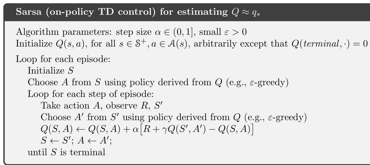

Q-learning off-policy control

If we let the target policy to be purely greedy, and still keep the behavior be $\epsilon$-greedy, then we get the Q-learning algorithm:

Deep Q-learning is recently used by DeepMind to play Atari games, Human-level control through deep reinforcement learning (2015).

Ex. 6.7: $$V_\pi(S_t) \leftarrow V_\pi(S_t) + \alpha [\rho_{t:t} (R_{t+1} + \gamma V_\pi(S_{t+1}))- V_\pi(S_t)]$$
Ex. 6.8:  \[G_t - Q_t(S_t, A_t) = \sum_{k = t}^{T-1} \gamma^{k-t}(1 + \gamma\alpha 1_{S_k = S_{k+1}, A_k = A_{k+1}})\delta_k\]

Ex. 6.9: With nine actions, the SARSA agent's behavior got worse, most likely due to its having extra action choices making it taking longer to learn, learning less reliable values, and thus mucking around for longer. I did not try eight actions, but my guess is that the agent would perform better in that case.

The optimal policy would make episodes last only 7 steps, but using 0.1-greedy policy, the average episode length converges to about 12. It shows that the optimal policy is not robust against randomness, and one misstep ruins the optimal policy.

Indeed, a rough calculation shows that the probability of executing the 7-step policy perfectly only has probability $(0.9 + 0.1/9)^7 = 52/%$. And some missteps would cost a lot more to fix, since it could cause the agent to wildly overshoot the goal if it's in the wind and have to make a big detour to get back to it. Still, 12 is better than 17, which is the the average episode length when there were only 4 actions available.

Ex. 6.10: It seemed significantly harder to complete this task for some reason. I tried using $\epsilon = 0.05$, which improved the agent so that it had an average episode length of 38.

Ex. 6.11: Because the behavior policy is exploratory, usually $\epsilon$-greedy, but the target polity is purely greedy.

Ex. 6.12: Assuming that the tie-breaking is the same, then yes.

What is TD(0) learning doing?

Consider "batch training", that is, instead of improving $Q$ during running, the agent simply play along without change and store all the game records, then after the games are over, learn on all the records all at once.

In batch learning, TD(0) is trying to approach the ideal of $V(S_t) = \mathbb{E}(R_{t+1} + \gamma V(S_{t+1}))$. Which is to say, the agent uses the game records to build a Markov chain model of the states and rewards, then calculate $V$ based on that model.

In contrast, batch learning MC is trying to minimize mean-squared error on the training set, without assuming that the environment is modelled by a Markov process.

This is a heuristic reason why TD learning works better on MPD problems.

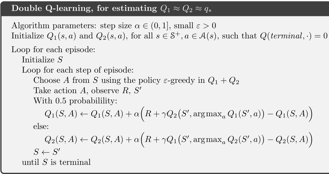
Too optimistic? Maximization Bias and Double Learning

The problem with control algorithms so far is that they are "too optimistic" in a sense. Imagine a Q-learning agent in Las Vegas, playing at a casino with 100 slot machines. Every one of them gives reward distributed normally, with mean $\$-1$ and std $\$ 10$. 

The agent starts by trying each one a few times. Just by blind luck, one of the slot machines gave the agent high payoffs several times, enticing the agent to keep playing for longer than it should. 

The problem is essentially that in the Q-learning algorithm, \[Q(S_t, A_t) \leftarrow Q(S_t, A_t) + \alpha\left[ R_{t+1} + \gamma\max_a Q(S_{t+1}, a) - Q(S_t, A_t) \right] \] the term \[\max_a Q(S_{t+1}, a) = Q(S_{t+1}, \underset{a}{\operatorname{argmax}}Q(S_{t+1}, a))\] used $Q$ twice, once in deciding which is the greediest action to do, once in estimating how good that action actually is. But asking $Q$ "How good do you think the best action, according to you, is?" is bound to cause some optimistic bias!

To deal with the problem, one way is "double learning". The basic idea is like this: two people are better than one person. So we would ask $Q_1$ to decide which would be the best action, and ask $Q_2$ to estimate how good that best action is.

Thus we get the double Q-learning, which turns out to be far more resilient to Las Vegas.

Ex. 6.13: The key step is this: 

\[Q_1(S, A) \leftarrow Q_1(S, A) + \alpha\left[ R + \gamma \sum_{a \in A(S')} Q_2(S', a) - Q_1(S, A) \right] \] \[\text{where}\quad \pi_1(a | S') = \begin{cases}1-\epsilon + \frac{\epsilon}{|A(S')|} \quad \text{if } a = \underset{a}{\operatorname{argmax}}Q_1(S',a),\\\frac{\epsilon}{|A(S')|}\quad \text{else}\end{cases}\]